This vignette describes the ways in which mapped forest stand data can be visualized using the forestexplorR package.
The size_dist() function can be used to produce and compare size-class distribution figures. contour_plot() uses measurements of any quantitative variable associated with coordinates to fit a contour map of that variable over a mapped stand. stand_map() produces a map of all trees in a mapped stand that can be used to navigate in the field.
size_dist(): Explore size-class distributions
The size_dist() function uses a tree census dataset to produce a size-class distribution of a specified stand. The most recent measurement of each tree in the census dataset is used to assign it to a size class. Below is an example of applying size_dist() to a single stand in the built-in tree dataset:
size_dist(size_data = tree, stands = "AB08")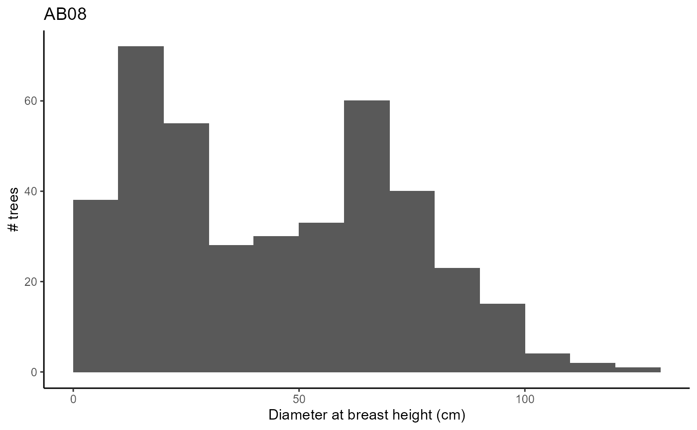
The default width of size-classes in the resulting plot is 10 dbh units, but can be changed:
size_dist(size_data = tree, stands = "AB08", bin_size = 5)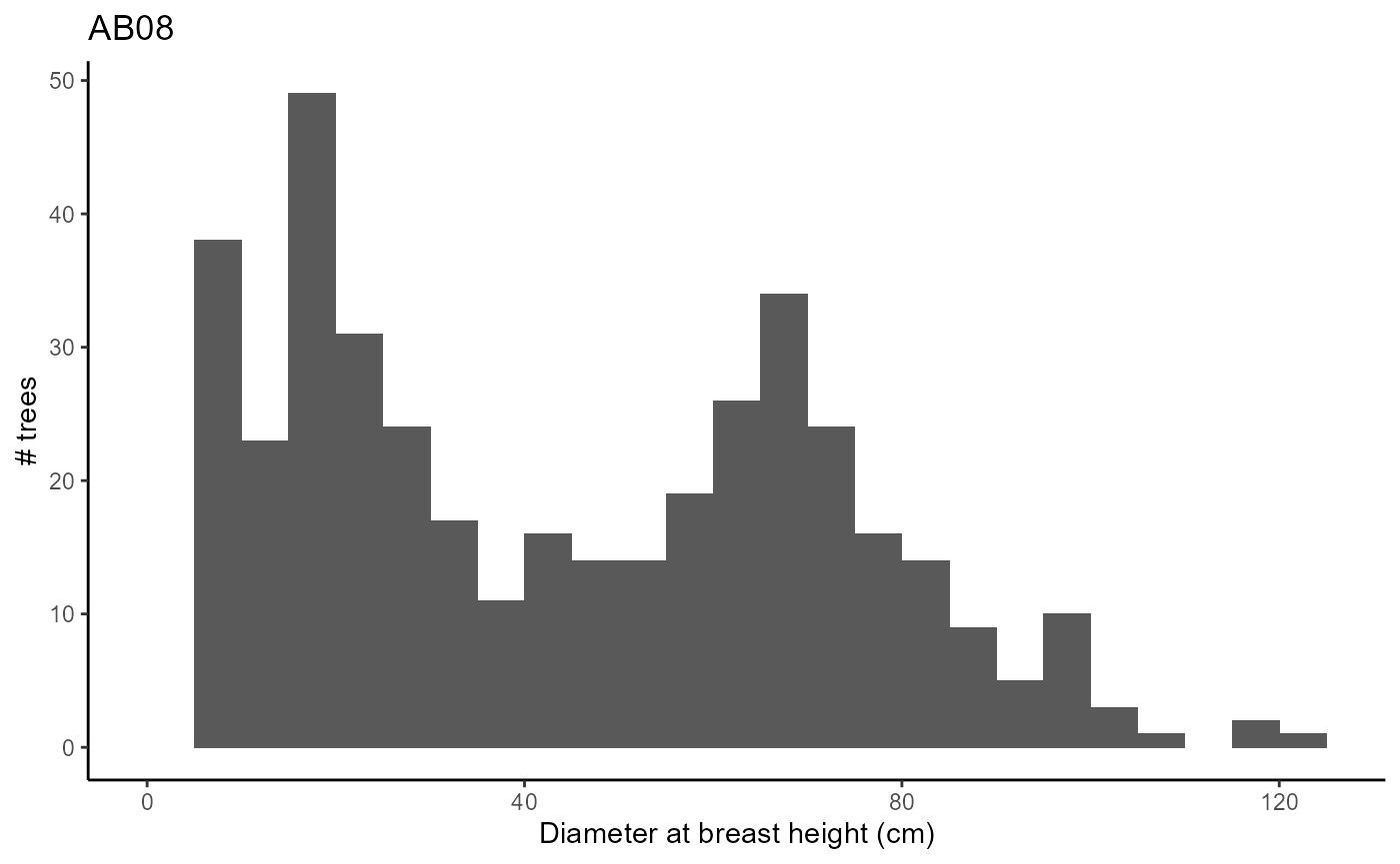
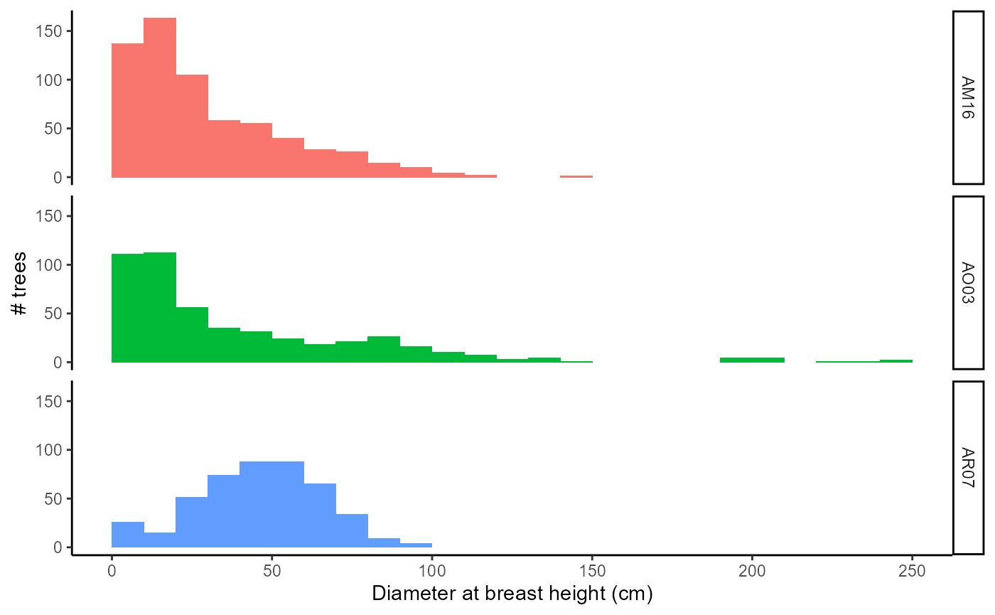
It is also possible to produce size-class distributions for multiple stands in order to compare them. To ensure clarity of individual distributions it is recommended that fewer than 10 stands be compared at once.
contour_plot(): Interpolate contours across stands
We often measure variables at known coordinates within mapped forest stands. If measurements are taken at enough locations, it may be desirable to interpolate the measured variable across the entire stand. This is the aim of the contour_plot() function.
With mapped forest stand data it is also possible to derive measurements at coordinate locations by calculating features of neighborhoods centered at those coordinates. As an example, here we will calculate tree density across a coordinate grid and create a contour plot of tree density.
First we create a grid of coordinate locations:
locations <- data.frame(
  loc_id = paste("A", 1:441, sep = ""),
  x_coord = rep(seq(0, 100, 5), times = 21),
  y_coord = rep(seq(0, 100, 5), each = 21))
Then we calculate tree density at each of these locations using forestexplorR functions:
nbhds <- neighborhoods(mapping, stands = "AB08", radius = 10,
                       coords = locations)
nbhd_summ <- neighborhood_summary(neighbors = nbhds, id_column = "loc_id",
                                  radius = 10, densities = "angular")
Next we join the coordinate locations with the calculated densities:
grid_data <- locations %>%
  left_join(nbhd_summ %>%
              select(loc_id, all_angle_sum),
            by = "loc_id") %>%
  select(-loc_id)
Now we can make the contour plot:
contour_plot(grid_data, "all_angle_sum", rad = 10, max_x = 100, max_y = 100)In the above plot, density appears to decrease toward the stand edges. This is because the locations close to the stand boundary did not have their entire neighborhood sampled. To improve the accuracy of values for these edge neighborhoods, we can use the edge_correction argument of neighborhood_summary(), which multiplies density values according to the proportion of the neighborhood area that lies beyond the stand boundary:
nbhd_summ <- neighborhood_summary(nbhds, id_column = "loc_id", radius = 10,
                                  densities = "angular", edge_correction = T,
                                  x_limit = 100, y_limit = 100)
grid_data <- locations %>%
  left_join(nbhd_summ %>%
              select(loc_id, all_angle_sum),
            by = "loc_id") %>%
  select(-loc_id)
contour_plot(grid_data, "all_angle_sum")
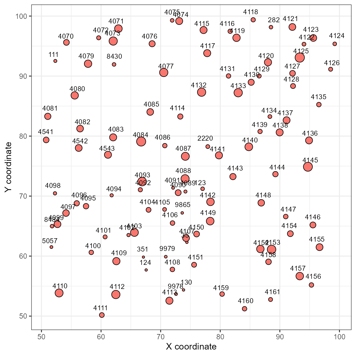
stand_map(): Create maps of forest stands
The stand_map() function creates a map of a forest stand with each tree represented by a point sized relative to its dbh and labeled with its tag number. The x and y coordinate limits must also be provided and can be used to create a map of only a portion of the stand:
# Isolate mapping and tree data for one stand
one_stand_map <- mapping %>%
  filter(stand_id == "AB08")
one_stand_tree <- tree %>%
  filter(stand_id == "AB08")

# Create stand map
stand_map(one_stand_map, one_stand_tree, c(50, 100), c(50, 100), "tag")